At Techtide Solutions, we tend to describe software as a set of promises: promises about speed, correctness, and how gracefully a system behaves when the world gets messy. Data structures are where those promises either become reliable habits—or brittle hope.
In our day-to-day work, “data structure” can sound academic until a production incident forces the issue: a slow search endpoint, a bloated memory footprint, a queue that suddenly backs up, or a billing job that turns into an all-night saga. Underneath the drama, the same question keeps surfacing: how are we representing information, and what operations are we forcing the machine to do repeatedly?
Across the public-cloud economy that hosts much of today’s data-intensive software, worldwide end-user spending is forecast to total $675.4 billion in 2024, and that scale is exactly why small structural choices in code can translate into meaningful infrastructure cost, latency, and customer experience.
Below, we’ll unpack what data structures mean, how they connect to algorithms, and how we apply them in real systems—because the best data structure is rarely “the fanciest,” and almost always “the one that matches what the product actually does.”
What is data structure? Meaning and core definition
1. Organizing and storing data for efficient access and use
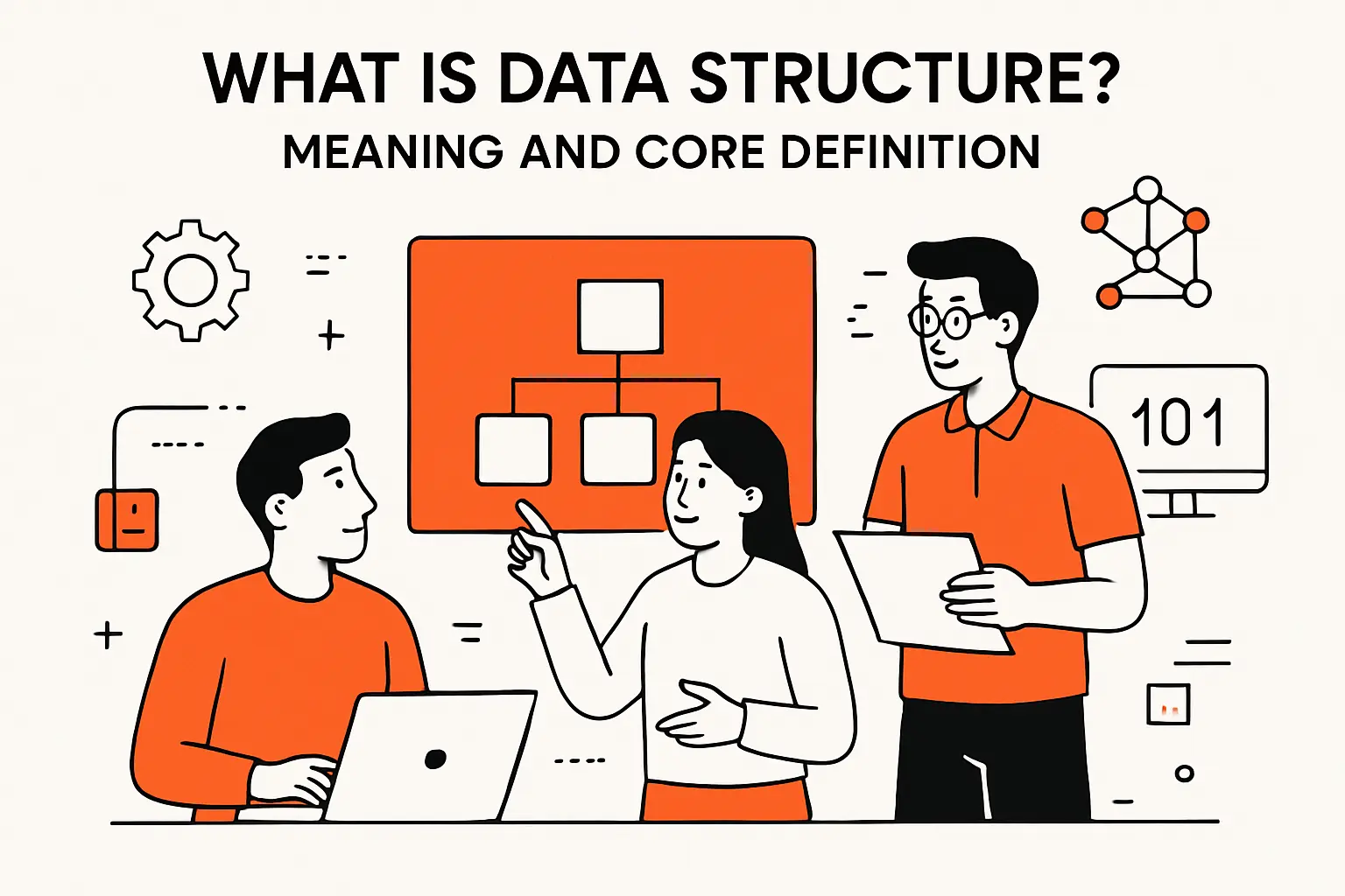
A data structure is a deliberate way of organizing and storing data so a program can access it and modify it efficiently. That efficiency is not just “speed” in a vague sense; it is the practical difference between an application that feels instant and one that feels sticky, between a backend that scales predictably and one that collapses under load.
From our perspective, the heart of the definition is intent. A plain pile of values in memory is not yet a useful structure. The moment we impose a shape—sequence, hierarchy, mapping, network—we are making a bet about which operations must be cheap and which can be expensive.
Why “shape” matters more than “storage”
In a customer-support tool, for example, “find all tickets assigned to this agent” is a frequent operation. If the data is stored only as a simple list, every query becomes a scan. If the data is also indexed by agent, the same operation becomes straightforward. Nothing “magical” happened; we simply chose a structure that matches the way the business uses the data.
2. Data values, relationships between values, and the operations applied to them
When we define a data structure well, we are defining three things at once: the data values we care about, the relationships among those values, and the operations we expect to perform. That triad is why data structures are not just containers; they’re operational contracts.
Related Posts
- Stacks and Queues Data Structures: Concepts, Operations, Implementations, and Use Cases
- What Is Big Data Analytics? Definition, How It Works, Tools, and Use Cases
- Impact Cycle Data Analytics: Turning Data into Actionable Insights with the IMPACT Framework
- Tree Data Structure: A Practical Guide to Concepts, Types, Traversal, and Uses
- Data Driven Decision Making: Benefits, Process, and Tools to Implement It
Consider a product catalog. The values are products and attributes. The relationships may include categories, variants, bundles, and “related items.” The operations could include filtering, faceting, deduplication, and ranking. A naive structure might treat everything as flat rows; a better structure might separate concerns so that a “variant group” behaves like a unit while still allowing per-variant availability.
Operations as the hidden requirements document
In practice, we often ask clients to describe their workflow verbs rather than their nouns. “Search,” “recommend,” “deduplicate,” “route,” “prioritize,” “expire,” and “audit” tell us more about the right data structure than “products,” “users,” or “events” ever will.
3. Logical representation and real implementation in a program
We distinguish between the logical representation of a data structure and its real implementation. Logically, we might want “a set of unique items,” “a queue of jobs,” or “a hierarchy of permissions.” Implementation-wise, we must decide how that structure lives in memory, how it is updated, and how it behaves under concurrency and failure.
This gap matters because the same logical structure can be implemented in multiple ways depending on language runtime, memory model, and performance goals. A “list” might be backed by contiguous memory, or it might be a chain of nodes. A “map” might be hash-based, tree-based, or even a sorted array with binary search. Each implementation comes with trade-offs that show up in profiling and incident reports.
Where abstraction helps—and where it hides costs
Modern languages offer friendly abstractions, and we love them for productivity. Still, abstractions can hide the difference between cache-friendly contiguous access and pointer-chasing scattered nodes. When performance matters, we treat the abstraction as a starting point, then validate the actual behavior with measurement.
Why are data structures important in programming?

1. Efficient processing of large and complex information
Software today rarely deals with tiny, toy datasets. Even modest products accumulate logs, events, customer records, messages, and derived analytics. As the information grows in volume and complexity, the data structure becomes the difference between “works in staging” and “works in the real world.”
Complexity is not only about size; it’s also about shape. A compliance engine may require traceability across entities. A logistics platform may require route constraints, time windows, and dependency chains. A personalization service may require fast joins between user context and item features. Each scenario pushes us toward structures that model relationships directly instead of forcing everything through repeated transformations.
Example: from raw events to actionable state
In event-driven systems, raw events are easy to append, but derived state is what the product needs. Choosing structures that support incremental updates—rather than full recomputation—often turns an “impossible” workload into a stable pipeline.
2. Improving performance through better storage and retrieval choices
Performance is not a single metric; it’s latency, throughput, memory, and predictability under load. Data structure choices touch all of them. A structure that is “fast on average” can still be a poor fit if its worst-case behavior aligns with peak traffic patterns, or if it triggers expensive memory allocations that amplify garbage collection pauses.
Under the hood, processors prefer predictable access patterns. Contiguous memory improves locality. Pointer-heavy structures can incur cache misses. Hash-based structures can be excellent for lookups, yet they may behave poorly if keys are adversarial or if resizing introduces latency spikes at inconvenient times. In our engineering practice, we treat these as design constraints, not trivia.
Performance as a product feature
Customers feel performance. Sales teams feel it too, especially when demos stutter. Choosing a structure that keeps “hot-path” operations cheap is one of the most direct ways to protect user experience without brute-forcing the problem with more infrastructure.
3. Supporting cleaner code through flexibility, reusability, and maintainability
Data structures are also about software design hygiene. When the structure matches the domain, code becomes simpler, and simpler code tends to be more correct. Instead of scattering ad hoc loops and filters everywhere, we encapsulate behavior: “enqueue,” “lookup,” “iterate children,” “merge,” “evict,” “index.”
Maintainability matters because requirements change. A system that begins as a small internal tool may become a customer-facing platform. If the underlying structures are clear and modular, new features tend to be additive. If the structures are muddled, every change becomes risky because it is unclear which invariants the code is relying on.
Flexibility without chaos
We aim for structures that evolve. That might mean using interfaces or abstract data types in our design, then swapping implementations when usage patterns become clearer. The key is to keep invariants explicit: uniqueness, ordering, allowed duplicates, or consistency rules.
Data structures and algorithms: understanding DSA
1. How data structures help algorithms run faster and use less memory
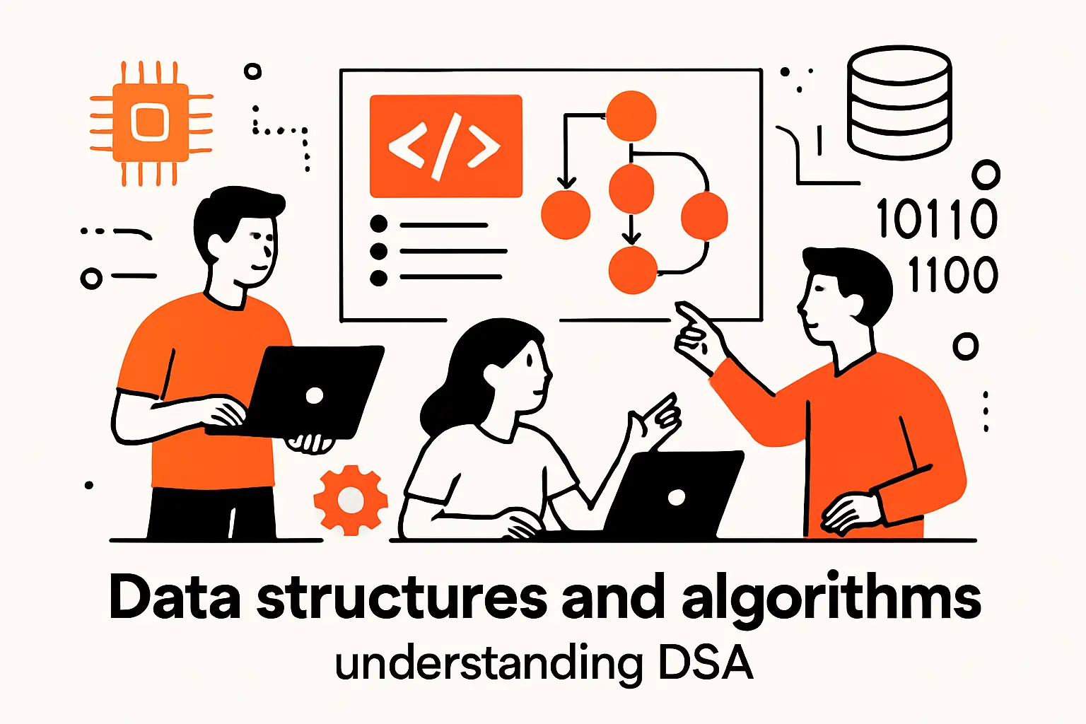
Algorithms are procedures; data structures are the stage they perform on. The same algorithmic idea can behave very differently depending on how the data is laid out. When we say “DSA,” we’re acknowledging that you rarely optimize one without understanding the other.
In search-heavy features, a well-chosen structure reduces the work an algorithm must do. In streaming pipelines, the right structure can reduce memory pressure by allowing incremental computation.And in concurrent systems, structure choices can reduce lock contention by partitioning state or by supporting mostly-read access patterns.
Practical example: caching and eviction
Many products need caching. The eviction policy is an algorithm, but the feasibility of that policy depends on structure. If we want to evict “least recently used” items, we need both quick lookup and quick reordering on access. That pairing pushes us toward a combined approach rather than a single primitive container.
2. Time complexity and space complexity as the core DSA challenges
In engineering conversations, the two core constraints are time and space. Time complexity is about how work grows as input grows. Space complexity is about how memory needs grow and how allocations behave. Even when the asymptotic story looks fine, constant factors and runtime realities can still dominate.
In our delivery work, we treat complexity analysis as a compass, not a GPS. It points us away from obviously bad choices, like repeatedly scanning a growing dataset inside a request path. Then profiling and observability tell us the truth about overhead: allocations, serialization, contention, and the cost of crossing network boundaries.
Why memory is a first-class constraint
Memory pressure causes cascading effects: more garbage collection, more paging risk, and more frequent scaling events. Selecting structures that avoid churn—especially in hot loops—often yields improvements that feel “too large to be real,” until you remember how expensive memory management can be at scale.
3. Dynamic programming and storing sub-solutions for reuse
Dynamic programming is a mindset: stop recomputing what you can store. The technique relies on representing partial results in a structure that supports fast retrieval, so future steps can reuse them. Without a suitable structure, dynamic programming degenerates into wishful thinking.
We see this pattern beyond textbook problems. Pricing engines reuse intermediate computations across similar carts. Recommendation pipelines reuse feature computations across sessions. Build systems reuse compilation artifacts. The common thread is deliberate memoization: choose keys that capture the state, store results safely, and invalidate them responsibly when inputs change.
Memoization in real products
In production, storing sub-solutions raises practical questions: how long should entries live, how do we bound memory, and how do we prevent stale results? Good structure choice is not only about lookup speed; it’s also about lifecycle management.
Common operations that drive data-structure choice

1. Searching, sorting, insertion, deletion, and indexing
Most data-structure debates are really operation-frequency debates in disguise. If an application frequently searches by key, we want direct access. If it frequently inserts new items, we want cheap mutation. And f it frequently needs ordered output, we want structures that preserve or can efficiently restore order.
Sorting is a special case because it can be either a one-time batch step or a constant requirement. In an analytics job, sorting might happen offline, so we can afford heavier computation. In an interactive UI—like a dashboard that needs to reorder results instantly—sorting strategy and representation matter much more.
Indexing as “pre-paying” for future queries
Indexing is a conscious trade: spend work during writes to make reads cheaper. Many businesses implicitly make this trade through database indexes, search indexes, and caching layers. Inside application code, the same logic applies when we maintain maps, sets, or grouped collections to avoid repeated scans.
2. Traversal patterns: sequential access, hierarchical navigation, and network exploration
Traversal is how software “walks” through data. Sequential access is typical for logs, feeds, and batch operations. Hierarchical navigation appears in menus, permission trees, org charts, and document structures. Network exploration shows up in dependency graphs, social graphs, routing, and recommendation neighborhoods.
Different traversals produce different performance profiles. Sequential traversal benefits from locality and streaming. Hierarchical traversal benefits from parent-child pointers and well-defined subtrees. Graph traversal benefits from adjacency representations that keep neighbors easy to enumerate without scanning unrelated edges.
Traversal shapes the API you expose
We often design the structure and the API together. If a caller needs “children of node,” the structure should support it naturally. If the caller needs “all reachable nodes under constraints,” we plan for that traversal up front, because bolting it on later can turn into a tangle of inefficient queries.
3. Big O notation as a practical way to compare performance trade-offs
Big O notation is a compact language for expressing how resource usage grows with input size. As practitioners, we use it to compare families of approaches and to avoid designs that will predictably degrade as data grows.
Still, we keep it grounded. A theoretically attractive structure can underperform if it causes poor locality, frequent allocations, or excessive indirection. Conversely, a “simple” approach can be excellent when input sizes are bounded or when the hot path benefits from tight loops and contiguous memory. For us, Big O thinking starts the conversation; measurement finishes it.
Trade-offs, not trophies
We never choose a data structure to win a trivia contest. The goal is to support the dominant operations cheaply, keep tail latency predictable, and preserve the ability to evolve the implementation without rewriting the product.
Linear data structures: sequential organization
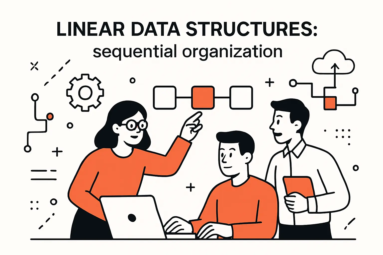
1. Arrays: contiguous memory, indexing, and common uses
Arrays represent sequential data in contiguous memory, which makes them naturally cache-friendly and fast for indexed access. When we need predictable iteration speed—processing a batch of events, rendering a list of UI elements, or applying a transformation to a collection—arrays are often the workhorse.
That said, arrays also have sharp edges. Insertions or deletions in the middle can be expensive because many elements must shift. Resizing can require allocating a new block and copying. In performance-sensitive paths, those costs can show up as latency spikes, especially when the array grows under load.
Where arrays shine in production systems
In data-processing code, arrays often power tight loops and vectorized operations. In backend services, arrays are useful for representing immutable snapshots: build once, read many times, and avoid churn by treating the collection as a stable value.
2. Stacks: last in, first out behavior and core operations
A stack models “last in, first out” behavior. Conceptually, it’s simple: push items on, pop items off, and the most recently added item is the next to be processed. That model matches many real tasks: parsing expressions, evaluating nested structures, undo functionality, and managing function call frames.
From an engineering viewpoint, stacks help enforce disciplined control flow. When we parse JSON-like inputs, for instance, a stack tracks the current nesting context. When we implement backtracking logic—say, in a rules engine—stacks naturally represent the decision trail.
Guardrails for stack use
Deep nesting can overflow call stacks in recursive implementations. In those cases, we often switch to an explicit stack structure in the heap so we can control growth, instrument behavior, and handle large inputs gracefully.
3. Queues: first in, first out behavior and core operations
A queue models “first in, first out” behavior, which is foundational for task scheduling and message processing. Jobs arrive, they wait their turn, and workers process them in arrival order. In distributed systems, this structure is practically a law of nature.
Queues appear at multiple levels: in-memory job queues, broker-backed message queues, and even user-visible concepts like “your requests are being processed.” The data structure matters because it determines how we handle backpressure, retries, and fairness. A naive queue can cause head-of-line blocking, where one slow task delays everything behind it.
Queues as product reliability tools
We design queue handling with failure in mind: idempotency, visibility timeouts, dead-letter routing, and safe acknowledgements. The queue structure is the backbone, but the surrounding invariants are what make it trustworthy.
Linked lists and pointer-based collections

1. Nodes and links: structure, navigation, and typical operations
Linked lists store elements as nodes connected by links, allowing efficient insertions and deletions when you already have a reference to the right location. Rather than requiring contiguous memory, they spread nodes across the heap, connecting them through pointers or references.
In real systems, linked lists show up in more places than people expect: maintaining an ordered set of active sessions, implementing certain cache eviction policies, building adjacency chains, or representing sequences where frequent splicing occurs. The ability to rearrange without shifting large contiguous blocks is the main advantage.
The hidden cost: indirection
Pointer chasing can be unfriendly to CPU caches. Each node may live far from the next, which can slow traversal compared to arrays. Whenever we consider a linked list, we ask whether the workload is mutation-heavy enough to justify the locality penalty.
2. Insertions and deletions vs random access trade-offs
The classic trade-off is simple: linked lists support cheap local edits, but they are poor for random access. If you need “give me the item at this position,” a linked list must walk node by node. Arrays, in contrast, excel at direct indexing.
In product terms, this becomes a question of user behavior and API usage. If a feature repeatedly scans a list end-to-end and rarely edits it, arrays or array-like lists tend to be superior. If the feature constantly splices, merges, or reorders, linked lists—or hybrid structures—can be the better fit.
Hybrid approaches we often prefer
In practice, we frequently combine structures: a map for direct lookup paired with a linked ordering for recency or priority. That pairing provides fast access while still allowing cheap reordering, which is a common need in caching, scheduling, and rate-limiting systems.
3. Structured aggregates in code: records, structs, and objects as ways to group data
Not all “data structures” are collections. Structured aggregates—records, structs, and objects—group related fields into a coherent unit. This matters for correctness and clarity: instead of passing parallel arrays or loosely related variables, we pass a single value that expresses meaning.
From a systems angle, aggregates define memory layout and serialization shape. In performance-sensitive code, field ordering and representation can affect cache behavior. In distributed systems, the aggregate becomes the payload contract, so stability, versioning, and backwards compatibility become part of the data-structure discussion.
Domain modeling as a data-structure decision
We treat “what fields belong together” as a first-class design decision. A well-modeled object can reduce bugs by making invalid states harder to represent, and it can make downstream algorithms simpler because assumptions are encoded in the structure itself.
Non-linear and associative data structures for relationships
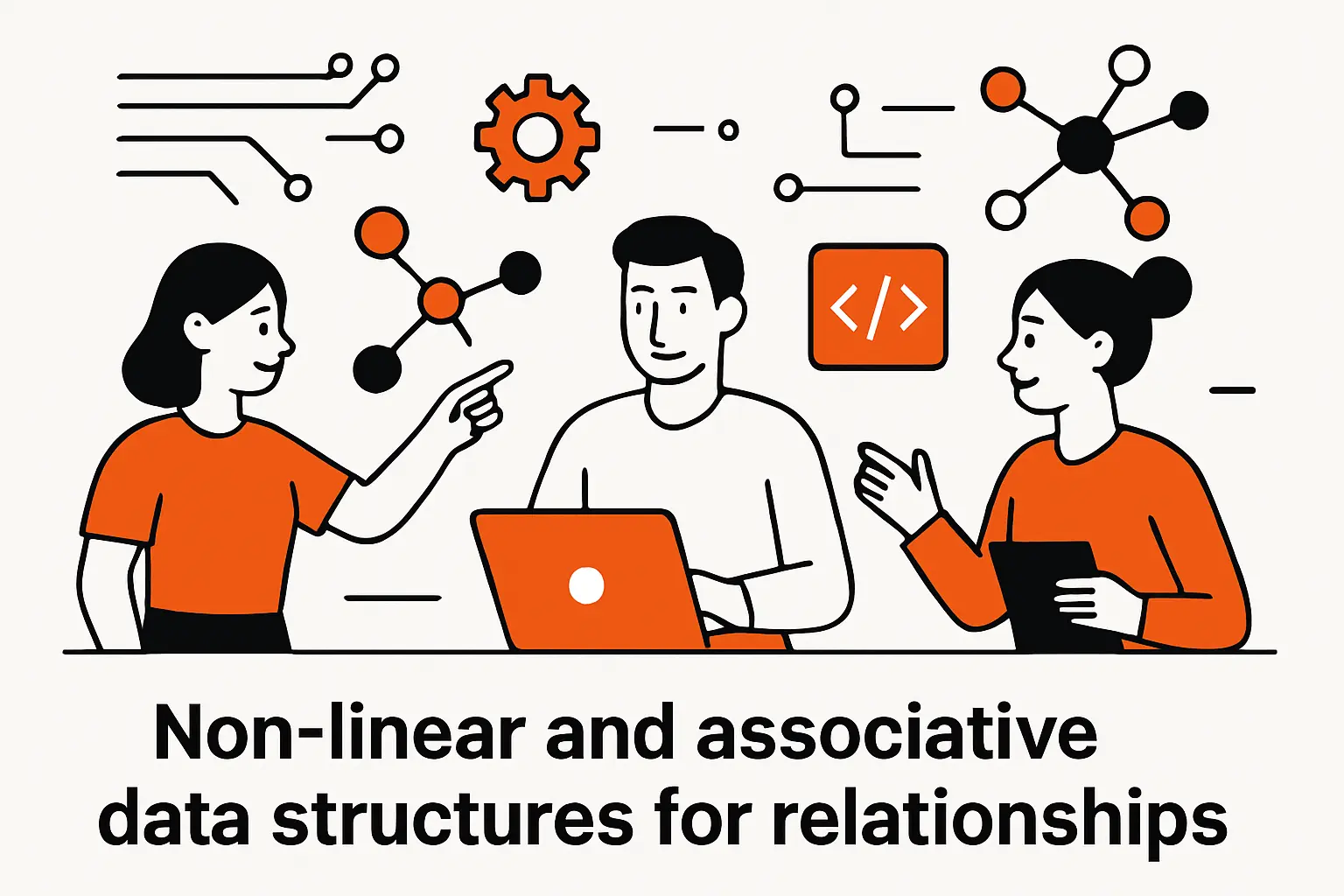
1. Trees: hierarchical structure, binary trees, and binary search tree ordering
Trees model hierarchical relationships: parent-child organization, nested containment, and scoped ownership. In product software, hierarchies are everywhere—categories, document outlines, org charts, permissions, configuration overlays, and UI component trees.
Binary trees are a familiar special case, and binary search trees impose an ordering that makes certain lookups efficient when the tree is balanced. In practice, we often encounter tree ideas in databases and storage engines through B-trees and related index structures, which are optimized for block storage and range queries.
Tree invariants are the point
The power of a tree comes from its invariants: ordering rules, balancing expectations, or structural constraints. When those invariants hold, algorithms become predictable. When they don’t, worst-case behavior can quietly creep in, which is why production-grade systems either enforce balancing or choose alternative structures for critical paths.
2. Graphs: vertices and edges for modeling connections and networks
Graphs model networks: entities as vertices and relationships as edges. Any time the question is “what is connected to what,” graphs are the natural mental model. Social connections, service dependencies, fraud rings, recommendation neighborhoods, and supply-chain relationships all fit.
Engineering graph features usually forces decisions about representation. An adjacency list representation is often efficient for sparse relationships and for exploring neighbors. Other representations can be better when connectivity is dense or when fast edge-existence checks dominate. The key is to choose based on traversal patterns and update rates.
Graph work is rarely just “in memory”
In real systems, graphs can be too large to fit comfortably in a single process. That pushes us toward storage-backed representations, caching strategies, and careful query planning. Even then, the underlying data structure choices inside the service still matter, because every request tends to touch the same hotspots.
3. Hash tables: key-value mapping, collisions, and fast average lookup
Hash tables map keys to values, aiming for fast average-case lookup, insertion, and deletion. They are the backbone of dictionaries and maps in many languages, and they power common product features like session stores, deduplication sets, routing tables, and in-memory caches.
Collisions are part of the deal: different keys can hash to the same bucket. Handling collisions well—through chaining or probing strategies—determines whether performance stays stable. Capacity management also matters; resizing at the wrong time can introduce latency spikes, so we design with growth patterns in mind.
Keys are an engineering decision, not a detail
Choosing keys sounds mundane until it breaks things. Poorly chosen keys can cause uneven hashing, expensive comparisons, or confusing semantics. In our systems, we prefer keys that are stable, canonical, and meaningful, because operational clarity is a form of performance too.
TechTide Solutions: custom software built on the right data structures
1. Performance-first engineering for scalable web apps and backend platforms
Performance-first engineering starts with a sober view of reality: web apps and backend platforms spend most of their time moving data—reading it, transforming it, indexing it, caching it, and shipping it across boundaries. Data structures are the lever arm that makes those movements cheap or costly.
In our delivery process, we begin by identifying hot paths and dominant operations. Observability signals—latency percentiles, allocation profiles, cache hit ratios, queue depth trends—tell us where the structure is fighting the workload. Then we change the representation so the common case is naturally efficient rather than “optimized” through scattered micro-tweaks.
How this looks in a typical web backend
For a search endpoint, we often separate “query-time work” from “ingestion-time work.” Index-like structures built during ingestion can reduce request-time computation. For a multi-tenant platform, partitioned maps and per-tenant structures can reduce contention and improve isolation.
2. Designing custom solutions by matching data structures to real product requirements
Custom software succeeds when it fits the product’s truth: the actual workflows, the real constraints, and the messy edge cases stakeholders forgot to mention. Data structures are where those truths become concrete. A system that must support audit trails needs append-friendly representations. A system that must support interactive filtering needs indexed structures. And a system that must handle bursts needs queueing and buffering that won’t collapse under pressure.
During design, we deliberately translate requirements into operations. “Users can edit and reorder items” implies mutation-friendly structures. “Users can search instantly” implies precomputed indexes and fast lookup. “Admins can apply rules to groups” implies efficient grouping and traversal. Once operations are clear, structure choices become far less mystical.
Real-world examples from our build patterns
- For notification pipelines, a queue-backed architecture prevents request threads from doing expensive downstream work synchronously, and it keeps failure handling explicit.
- In recommendation features, associative structures support fast feature retrieval, while graph-like representations express “relatedness” more naturally than flat tables.
- Within authorization systems, tree-shaped role inheritance and scoped permission evaluation keep policy logic understandable instead of turning it into scattered conditional checks.
3. Refactoring and optimizing existing systems for maintainability, speed, and efficient resource use
Most organizations don’t start from scratch, and we rarely recommend that they do. Refactoring existing systems is often the highest-leverage route, especially when the business logic is correct but the performance and maintainability are slipping.
In refactors, we look for structural smells: repeated scans over the same collection, expensive transformations performed per request, or “god objects” that try to represent everything at once. Frequently, the fix is not a clever algorithm; it is a better data structure that allows the straightforward algorithm to run efficiently.
Our typical optimization playbook
First, we measure to avoid superstition-driven rewrites. Next, we isolate the problematic component behind a clear interface so we can safely swap implementations. Finally, we validate improvements with realistic load tests and production telemetry, because the goal is durable behavior, not a one-off benchmark win.
Conclusion: applying what is data structure knowledge in practice
1. Start with the data you have and the operations you need to perform most
In practice, the best starting point is not a catalog of structures; it is a clear inventory of operations. What do we read most? What do we write most? Which queries are on the request path, and which can run asynchronously? Where do we need ordering, uniqueness, grouping, or fast neighbor lookup?
Once those questions are answered, many decisions become obvious. A system dominated by membership checks calls for set-like behavior. A system dominated by ordered traversal calls for order-preserving structures. And a system dominated by “find by key” calls for mapping. The workload tells the story if we listen closely enough.
A question we ask clients early
Instead of “what data do you store,” we ask “what do you do with it every day?” That shift keeps architecture aligned with business reality and prevents beautiful structures from being built for imaginary usage patterns.
2. Choose structures that balance runtime, memory usage, and implementation complexity
Every data structure is a bundle of trade-offs. Faster reads may require heavier writes. Lower latency may require higher memory overhead. Cleaner abstractions may hide costs that become painful at scale. The right choice depends on constraints and on the maturity of the system.
From our viewpoint, implementation complexity is an underappreciated dimension. A theoretically optimal structure that only one engineer understands is a liability. We prefer designs that are robust, testable, and debuggable, even if they are not “perfect” in a textbook sense, because production software must survive change.
How we make trade-offs explicit
We document invariants, expected operation costs, and failure modes alongside the structure. That habit turns “tribal knowledge” into shared understanding, and it makes future refactors safer because the next team can see what the original structure was protecting.
3. Build DSA intuition by pairing each data structure with the algorithms that manipulate it
DSA intuition grows when structures and algorithms are learned together, as a pair. A structure without its typical algorithms is just a container. An algorithm without a structure is often a slow idea waiting to happen. Pairing them teaches the important lesson: most performance improvements come from aligning representation with behavior.
In our own practice at Techtide Solutions, we encourage teams to build small mental templates: “If we need fast lookup, we reach for a map and design good keys.” “If we need ordered ranges, we reach for an ordered structure and preserve its invariants.” “If we need network exploration, we represent neighbors explicitly and optimize traversal.” That’s not dogma; it’s a starting point for thoughtful engineering.
So what’s the next step for your codebase: should we profile your hottest endpoints and identify the structures doing unnecessary work, or should we review a new feature’s operations early enough to choose a representation that will still feel effortless when usage grows?


