In our work at Techtide Solutions, we treat a tree as the most honest way to model “real life” structure in software: managers and reports, folders and files, categories and products, syntax rules and expressions. Unlike arrays or linked lists, a tree branches, and that branching is exactly the point—there is more than one “next” option, so the structure cannot be reduced to a single straight line without losing meaning.
What is a tree data structure
1. Hierarchical parent–child relationships and why trees are non-linear
Because of that branching, trees are called non-linear data structures. Multiple paths can exist from the top of the structure toward different outcomes, and the interesting questions tend to be about navigation: “Which branch do we follow?” and “How do we visit everything without missing anything?” From a business lens, that same non-linearity shows up as decision rules, nested permissions, product bundles, dependency graphs that have been simplified into hierarchies, and user journeys that fork based on intent.
So when we say “tree,” we are really saying “hierarchy with rules.” Once a system has hierarchy, the core engineering job becomes preserving those rules while still enabling fast lookups, safe updates, and predictable behavior under load.
2. Nodes, edges, and the root as the organizing structure
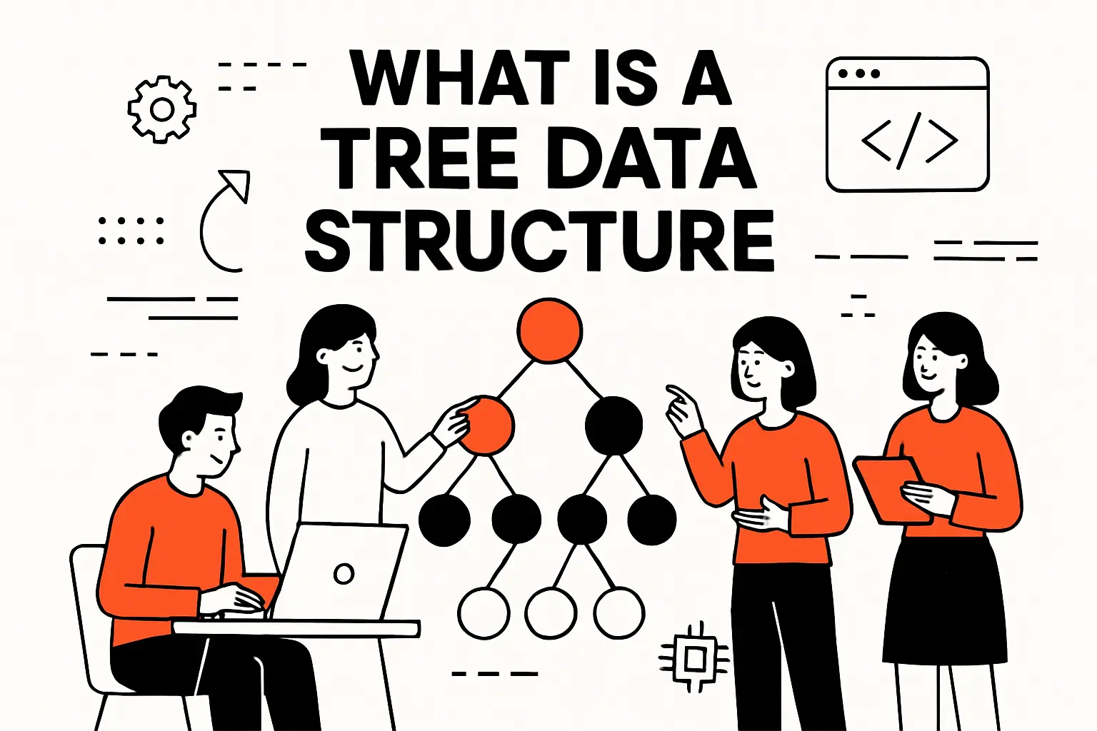
A tree is composed of nodes (the “things”) and edges (the “relationships”). Put differently, nodes store the payload—an ID, a label, a configuration, a computed value—while edges encode how one node connects to another. In day-to-day engineering, we usually represent an edge as a reference, pointer, or index from a parent node to its child node.
The root node is the organizing anchor. Practically, it becomes our entry point: the one object we already have, from which we can reach everything else by following references. That property matters because software is fundamentally about reachability; a structure is only useful if our runtime can reliably get from what it knows to what it needs.
Market context helps explain why trees keep showing up in production systems: database platforms and the services around them keep growing, and Gartner forecasts worldwide DBMS spending to reach 3.6 billion by 2027, which means more teams will be building features where indexing, hierarchical access patterns, and predictable retrieval costs are not “nice-to-haves,” but core product requirements.
3. Core constraints: one parent per node, no cycles, and connected subtrees
The constraints of a tree are what make it powerful. In a typical rooted tree, every node (except the root) has exactly one parent. That single-parent rule gives us a unique upward path from any node to the root, which becomes the backbone for operations like permission inheritance, breadcrumb navigation, and “roll up” analytics.
No cycles are allowed, meaning we cannot start at one node and follow edges and eventually come back to the same node. From an operational standpoint, cycle-free structure is a safety feature: it prevents infinite loops during traversal, makes reasoning about ancestry unambiguous, and allows “subtree” to have a precise meaning rather than a fuzzy one.
Related Posts
- Stacks and Queues Data Structures: Concepts, Operations, Implementations, and Use Cases
- What Is Big Data Analytics? Definition, How It Works, Tools, and Use Cases
- Impact Cycle Data Analytics: Turning Data into Actionable Insights with the IMPACT Framework
- Data Driven Decision Making: Benefits, Process, and Tools to Implement It
Connectivity is the other quiet constraint: in a tree, all nodes are reachable from the root if we follow edges in the allowed direction. That requirement sounds abstract, yet it is exactly why trees are useful in software architecture—if the structure can fragment into unreachable islands, it stops being a coherent model of the system we are trying to represent.
Essential tree terminology for beginners
1. Node, edge, and pointers or references between nodes
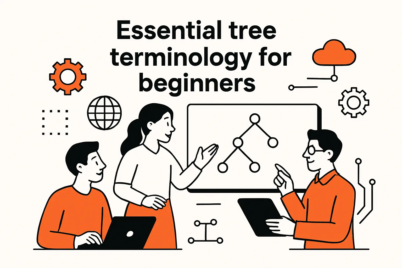
When we introduce tree concepts to new engineers on our team, we start with the vocabulary that maps cleanly to code. A node is typically an object or struct. An edge is typically a field inside that object pointing to another node, or an entry in a collection of children. That “edge as a reference” framing is not academic; it directly influences memory layout, garbage collection pressure, and how we reason about mutation.
In managed runtimes, references are often safe and convenient, but they can scatter nodes across memory. In lower-level environments, pointers can be fast but demand discipline around ownership and lifetimes. Across both styles, the edge is still the same conceptual idea: the mechanism that lets one node lead us to another.
From a system-design angle, we also watch how edges are stored because it changes performance characteristics. A node that stores children in a dynamic array tends to favor iteration, while a node that stores children in a map tends to favor keyed access, and a node that stores children in a linked structure tends to favor cheap insertions at the cost of locality.
2. Parent, child, sibling, and neighbor relationships
Parent and child relationships are the directional meaning of an edge: the parent owns the link, and the child is the destination. Once that exists, sibling relationships become emergent: siblings are nodes that share the same parent. In business systems, siblings often translate into “items under the same category,” “users under the same organization,” or “steps within the same workflow stage.”
Neighbor is a more context-dependent term. In an ordered tree, neighbors can mean “adjacent siblings” according to a defined sequence. In an unordered tree, “neighbor” might mean “some node in the same local region of the hierarchy,” which matters in UIs that show “next/previous” navigation or in algorithms that perform local balancing and rotations.
And in practice, we choose terminology that matches the product’s mental model. A taxonomy editor might care deeply about sibling order, while a permission system might care only about ancestry. The structure is the same, yet the language we emphasize changes what engineers optimize and what testers verify.
3. Ancestor, descendant, and subtree concepts
Ancestor and descendant relationships let us talk about reachability along parent pointers (or implied parent pointers) rather than only along explicit child pointers. An ancestor of a node is any node on the path from that node up toward the root, and a descendant is any node that lives below it. That “path” concept is the bridge from vocabulary to algorithms.
A subtree is the most operationally important abstraction: pick any node, and the node plus all its descendants form a subtree. In our experience, that is how real features get implemented. When a customer disables a department, we disable the entire subtree of teams. When a merchant unpublishes a category, we unpublish the entire subtree of products. And when a build pipeline invalidates a target, it often invalidates the subtree of dependent steps.
Once subtree operations enter the product, engineering decisions start to matter: do we compute ancestor paths on the fly, store materialized paths, maintain “closure tables,” or use specialized indexes? Trees feel simple until the business asks for bulk operations, audit logs, and guarantees around consistency.
Tree properties and measurements: level, degree, depth, height, size
1. Levels and distance as edge counts along paths
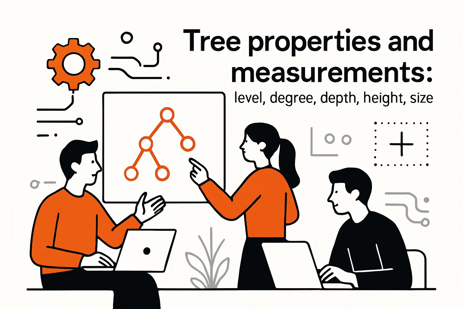
Level is a way to talk about “how far down” a node is, and distance is a way to talk about “how far apart” two nodes are, typically measured in edges along a path. Conceptually, we imagine the root at the top, then children below it, then grandchildren below that. That visual metaphor is surprisingly practical because it matches how teams think about navigation menus, nested settings, and organization charts.
Distance matters anytime we need the shortest route within the structure. In permission inheritance, for example, the closest applicable policy might win. In UI rendering, the distance from the root can determine indentation, breadcrumb length, and whether we collapse intermediate nodes.
From a performance standpoint, levels matter because traversal cost grows with the number of edges we must follow. Even when each pointer hop is cheap, lots of hops amplify cache misses and latency variance. That is why, in production systems, we often try to keep “hot” queries from depending on walking very deep paths.
2. Degree of a node vs degree of the entire tree
The degree of a node is the count of its children. A node with many children is “wide,” while a node with one child behaves more like a linked list. The degree of the tree is usually the maximum degree among all nodes. Although these terms can sound academic, they map directly to system behavior.
Wide nodes tend to stress iteration and storage of child collections. If children are stored in arrays, updates can become expensive when insertion requires shifting. If children are stored in hash maps, memory overhead can rise. And if children are stored in balanced structures, the overhead can be justified by fast searches among children.
In product work, “wide” nodes show up all the time—catalog menus, multi-tenant admin dashboards, or analytics views where one parent owns a huge pile of items.
Our bias is simple: measure the real shape of your data early. The degree distribution (how many children each node has) tells you what to optimize for. If access is breadth-heavy, you’ll care about batching, pagination, and caching. If it’s depth-heavy, you’ll lean toward tricks like path compression and fast ancestor lookups.
3. Depth vs height and how overall tree height is defined
Depth is typically defined per node: how many edges from the root to that node. Height is often defined as the maximum depth among all nodes, or as the longest downward path from a node to a leaf, depending on the textbook. In implementation conversations, we make the definition explicit because ambiguity here can quietly create off-by-one errors in traversal, layout, and balancing logic.
A tall tree means searches go deeper and recursive code can run into big call stacks. A short tree means more branching at each level, so you may spend more time scanning lots of children. Neither is “better” universally; the right shape depends on the access pattern.
In business features, height shows up in constraints: how many nested categories do we allow, how many nested folders can exist, how many nested rules can be composed before the UI becomes unreadable? Engineering and product meet here, because height is as much a usability question as it is a runtime question.
4. Forests and how disjoint trees can be formed from a tree
A forest is a collection of disjoint trees. Forests appear naturally when we remove a root, detach subtrees, or treat each top-level entity as the root of its own hierarchy. In enterprise software, a multi-tenant system often behaves like a forest: each tenant has its own tree of resources, policies, and content.
Operationally, forests matter because they change how we store and query. If we have many small trees, we might shard by root and scale horizontally. If we have one huge tree, we might focus on indexing and caching within a single logical namespace. Either way, we need to answer the same core question: given an arbitrary node ID, how do we find its root and ensure we operate within the correct tree?
In our delivery work, forests also show up as a migration pattern. A monolith might start with a single shared hierarchy, then later split into per-customer roots for isolation, compliance, and performance predictability. Designing for that split early saves painful refactors later.
Types of trees and how they are classified
1. Rooted vs unrooted trees and ordered vs unordered children
A rooted tree has a designated root that defines direction: parents lead to children. An unrooted tree is more like a pure connectivity structure with no special starting node. In everyday software engineering, rooted trees dominate because applications need a stable entry point and a consistent interpretation of “up” versus “down.”
Ordered versus unordered children is a classification that sounds trivial until the UI team asks for drag-and-drop ordering, or the API contract requires stable pagination. An ordered tree treats the sequence of children as meaningful, so sibling order becomes part of the data model. An unordered tree treats children as a set, so order is either undefined or derived.
From a storage perspective, ordered trees push us toward arrays or lists plus explicit position metadata, while unordered trees can lean on sets or maps. In our systems, the decision hinges on what needs to be stable: user intent (order matters) or structural membership (order does not).
2. Binary, ternary, and N-ary trees as child-count classifications
Child-count classifications define the maximum number of children a node can have. Binary trees restrict nodes to at most two children, which is why they have such a rich ecosystem of algorithms: the constraint makes balancing and traversal patterns tractable. Ternary and general N-ary trees loosen that constraint, often matching real-world hierarchies more naturally.
In product modeling, N-ary trees are common: a category can have many subcategories, a folder can have many files, a UI component can contain many children. So while binary trees are iconic in interviews, N-ary trees are often the ones paying rent in production.
Implementation choices shift with arity. A binary tree can store two direct child references, which is compact and predictable. An N-ary node often stores a dynamic collection, and that opens design questions around ordering, deduplication, concurrency, and whether we optimize for reads or writes.
3. Common binary tree shapes: full, complete, balanced, perfect
Binary tree “shapes” describe structural properties that influence performance. A full binary tree typically means each internal node has either two children or none, which removes certain irregularities. A complete binary tree is filled level by level from left to right, which is why it maps cleanly to arrays and is popular for heaps.
Balanced is the practical goal in search trees: we want height to remain small relative to the number of nodes, so operations stay fast and predictable. Perfect is an idealized shape where every level is fully filled, which rarely holds in dynamic systems but serves as a helpful reference point.
In real services, shape is not just theory; it is uptime. A search structure that quietly drifts into a pathological shape can turn a stable endpoint into a latency outlier. That is why production-grade tree structures typically include balancing rules, randomized behavior, or rebuild strategies to keep shape under control.
Specialized trees used for efficient search and storage
1. Binary search trees: ordering rules and search-oriented structure
A binary search tree (BST) adds an ordering rule: values in the left subtree compare “less than” the node, and values in the right subtree compare “greater than.” That rule turns the tree into a navigable decision structure, where each comparison lets us discard half the remaining search space—at least when the tree stays reasonably balanced.
In business systems, the BST idea generalizes beyond primitive values. Once we define a comparator for our domain (timestamps, lexicographic keys, composite identifiers), the tree becomes a way to keep data sorted while still supporting inserts and deletes. That is why ordered indexes are so central to databases and search-heavy APIs.
Across our back-end engagements, we also treat “ordering rules” as governance. If the comparator changes, the tree’s meaning changes. Consequently, schema evolution, locale rules, and case sensitivity become correctness issues rather than mere formatting details.
2. Self-balancing search trees: AVL trees and red-black trees
Self-balancing trees exist because naïve BSTs can degrade when inserts arrive in already-sorted order, producing a tall structure that behaves like a linked list. AVL trees and red-black trees impose invariants that keep height bounded by enforcing rotations and color or balance-factor rules during updates.
AVL trees keep a tighter balance, so lookups can be a bit faster, but writes often pay more rebalancing work. Red-black trees allow slightly looser balance, which usually means fewer rotations during inserts and deletes.
In system terms, it’s a classic trade: read-heavy workloads often like AVL; write-heavy workloads often prefer red-black. The real question is whether you can tolerate occasional write latency spikes—or if you want writes to stay smoother even if reads are a tiny bit less optimal.
Operationally, the most important lesson is not the exact invariants, but the design pattern: make structural correctness enforceable locally during updates. That “local repair” principle scales across many data structures and prevents global rebuilds from becoming routine maintenance.
3. Multiway and index-oriented trees: B-trees and B+ trees
B-trees and B+ trees are designed for storage systems, especially those involving disks or SSDs, where the cost of fetching a block dwarfs the cost of comparing in memory. Instead of limiting each node to two children, these structures store many keys per node, which reduces height and minimizes expensive I/O.
B+ trees push values to leaves and keep internal nodes as routing tables, which makes range scans efficient and predictable. That design explains why B-tree-family indexes show up repeatedly in databases and filesystems: they can serve both point lookups and ordered traversal without forcing a separate structure.
In practical engineering, we also care about how these trees behave under concurrency. Latching strategies, page splits, and defragmentation policies determine whether an index remains stable under mixed workloads. When a product manager says “we need sorted retrieval plus fast inserts,” the B-tree family is usually where we start our mental search.
4. Other practical variants: heaps, tries, and spatial trees such as quadtrees and octrees
Heaps are tree-based structures built to grab the smallest or largest item quickly. Their superpower is prioritization, so they show up in schedulers and task queues, job dispatchers, timed event systems, and anything where “what should run next?” is the core question.
In practice, heaps often sit behind features like “fairness” and “responsiveness.” Users don’t see the heap, but they feel it—when the app stays snappy, when urgent work jumps the line without starving everything else, and when the system behaves like it has manners instead of mood swings.
Tries organize strings or tokens by shared prefixes, which makes them a natural fit for autocomplete, routing tables, and dictionaries. When we build search experiences, tries often outperform ad hoc approaches because they encode the domain’s shape—prefix overlap—into the structure itself.
Spatial trees like quadtrees (2D) and octrees (3D) organize space so you can ask questions like “what’s near this point?” without checking everything.
That’s why rendering engines, collision detection, maps, and simulations lean on them—they avoid the slow, brute-force “compare against every object” approach. In business systems, the same trick shows up in logistics routing, geofencing, and even UI hit-testing for busy interactive canvases, where you want clicks to land accurately without your app wheezing.
Traversal and core operations in the tree data structure
1. Why traversal is required to reach and operate on specific nodes
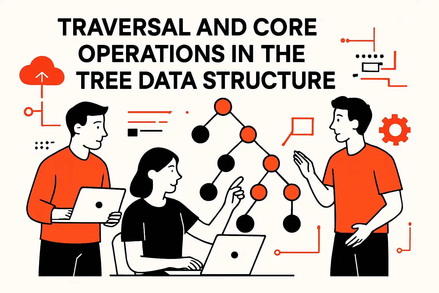
Traversal is how we turn a tree from a static shape into an operational tool. Because nodes are connected via edges rather than arranged in a contiguous line, we cannot “just index” into the structure without a plan. Instead, we define a strategy for visiting nodes in some order, and we use that visit order to compute results, apply updates, or collect data.
Traversal is everywhere in product work. “Show me everything in this folder” is traversal. “Recompute totals for this category and all subcategories” is traversal. Even “render the UI component tree” is traversal—so frontend performance often comes down to skipping unnecessary walks through the component hierarchy.
From our delivery perspective, the key is to match traversal to intent. If we only need a single node and have an index, a full traversal is waste. If we need to validate invariants across a hierarchy, traversal is unavoidable, so we focus on pruning, caching, and incremental recomputation.
2. Depth-first traversal: pre-order, in-order, post-order
Depth-first traversal explores a branch as far as it can before backtracking. Pre-order visits a node before its children, which is ideal when we want to serialize structure, copy a tree, or emit a representation where parents must appear before descendants. In-order is specific to binary trees and yields sorted output when applied to a binary search tree, which is why it is often taught as the “ordered traversal.”
Post-order visits children before the parent, and that pattern is invaluable when we need to delete a subtree safely or compute derived values that depend on children. Build systems and dependency evaluation often behave like post-order traversals: compute prerequisites first, then compute the target.
In our code reviews, we look for clarity more than cleverness. Depth-first logic tends to be concise, yet it can hide costs if it walks large subtrees repeatedly. So we often pair depth-first traversal with memoization, explicit stacks for better control, or instrumentation that makes traversal frequency visible in production telemetry.
3. Breadth-first traversal: level-order visiting
Breadth-first traversal visits nodes level by level. A queue usually drives the process: you visit the current node, enqueue its children, then process nodes in the order you discovered them. This traversal mirrors how people often think about hierarchies: top-down, expanding outward.
In real systems, breadth-first traversal is useful for “nearest match” problems, like finding the closest applicable policy, or for UI rendering scenarios where we progressively load shallow content before deep content. It also helps in scenarios where we want to cap work: we can stop after certain levels, which provides a natural throttle in user-facing APIs.
Under load, breadth-first can have a different memory profile than depth-first because it may hold many nodes from a wide level in memory at once. That is not inherently bad, but it becomes a design consideration in trees with high branching factors, particularly when nodes are heavy objects rather than lightweight references.
4. Common operations: search, insert, delete, prune, graft, and lowest common ancestor
Tree operations map closely to business actions. Search is “find the node.” Insert is “add a new child or subtree.” Delete removes a node, and your rules decide what happens next—do you delete the children, reattach them, or promote them? Pruning drops an entire subtree. Grafting attaches a subtree somewhere new, like when someone drags a folder into another folder or reshuffles an org chart.
Lowest common ancestor (LCA) sounds theoretical, yet it shows up in permissions (“what policy applies to both of these resources?”), navigation (“where do these two items meet in the hierarchy?”), and analytics (“what category contains both of these products?”). Efficient LCA strategies matter when systems must answer such questions repeatedly at scale.
In production, correctness rules dominate: preventing invalid moves, enforcing constraints, and maintaining indexes. That is why we prefer to design tree operations as transactional units with explicit invariants, rather than letting scattered parts of the codebase mutate pointers freely.
Implementing trees in code and deciding when to use them
1. Node-based implementations: storing values plus child references
A node-based implementation is the most direct: each node stores its value and references to its children. For binary trees, that might be left and right references. For N-ary trees, it is usually a collection such as a list or vector. The flexibility comes from this: you can create, remove, and reorganize nodes without moving one big, continuous block of memory.
In our implementations, we pay close attention to ownership. If multiple places can reference the same node, you’re no longer modeling a strict tree—you’re drifting into a directed acyclic graph. That shift might be correct for some domains, but it changes the invariants. For strict trees, we often enforce a single-owner model and expose safe operations for moving subtrees.
Debuggability matters too. You can inspect node-based trees with logging and visualization tools, and they match how developers naturally reason about objects. When a production incident occurs, that clarity becomes a competitive advantage.
2. Array-backed representations and when contiguous layouts can help performance
Array-based trees store nodes next to each other in memory, and they usually use simple position rules to find a node’s parent and children. A heap is the most common example. This layout is compact, works well with the CPU cache, and is quick to move through for tasks such as scheduling. Because related data stays close together, it can use memory more efficiently than storing many separate objects, especially in languages or runtime environments where creating and cleaning up many objects is expensive.
That speed comes with limits. Array-based trees usually work best when the tree follows a fixed pattern, as heaps do. Adding or removing items in random places can be costly if many elements have to be moved or if the structure needs to be rebuilt often.
In our system design, we choose array-based layouts when the tree’s form does not change much and high speed is important. On the other hand, if the product frequently re-parents nodes, moves large sections of the tree, or deals with unevenly distributed branches, a node-based approach is usually simpler and less error-prone.
3. Recursion as a natural fit for tree algorithms and scalable problem decomposition
Recursion matches trees because a tree is self-similar: each subtree is a smaller tree. That property makes many algorithms elegant, readable, and directly tied to the definitions we use when we reason about correctness. For example, “compute the size of a tree” naturally decomposes into “one plus the sizes of the children.”
Still, recursion is not automatically safe at scale. Deep trees can cause stack overflows in environments with limited call stacks, and heavy recursion can obscure performance costs when it is mixed with expensive per-node work. When we anticipate deep hierarchies, we often switch to explicit stacks or iterative traversals while preserving the same conceptual structure.
From an engineering culture standpoint, recursion is a litmus test for clarity. If recursive code is hard to understand, the underlying model might be poorly defined. When recursive code reads cleanly, it usually indicates the data model and invariants are aligned with the domain.
4. Where trees show up in real systems: file systems, DOM and XML/HTML, syntax trees, databases, routing, scheduling, and rendering
File systems are an obvious tree: directories contain files and other directories, with a root anchoring the namespace. Frontend development is equally tree-centric: the DOM Standard models documents as a tree of nodes, which is why rendering, event propagation, and UI updates often feel like tree problems wearing browser clothing.
XML and HTML parsers build parse trees, and compilers build syntax trees to represent code structure before optimization and code generation. Databases rely on tree-based indexes for ordered access and range queries; as a concrete anchor, the PostgreSQL documentation on index types describes how B-tree-family indexes support common query patterns in practice.
Routing tables and naming systems also carry tree DNA. DNS, for instance, is built around a hierarchical namespace described in Domain Names—Concepts and Facilities, and that hierarchy shapes how resolution, delegation, and caching work. Scheduling and rendering frequently depend on priority structures and spatial partitioning trees, turning “data structures” into direct determinants of user experience.
TechTide Solutions: Building custom solutions with the tree data structure
1. Custom web and mobile apps that model hierarchical customer and product data
Hierarchies are a recurring theme in the applications we build. Customer accounts often contain organizations, organizations contain teams, teams contain roles, and roles contain permissions. Product catalogs follow a similar shape: departments contain categories, categories contain subcategories, and leaf categories contain items with variants, bundles, and localized content.
In these systems, the hard part is rarely “store the tree.” The harder part is keeping the tree consistent while enabling edits that feel instantaneous in the UI. Drag-and-drop reordering, subtree moves, bulk updates, inherited attributes, and audit history all stress the same underlying requirement: operations must be safe, expressive, and performant.
Our preferred approach is to model the domain with explicit invariants, then choose storage and traversal strategies that support the business workflow. That might mean a straightforward adjacency list in a relational database for modest scale, or it might mean materialized paths, closure tables, or specialized search indexes when analytics and access control become dominant.
2. Performance-focused back-end services using tree-based indexes and retrieval strategies
Backend performance is often an indexing story, and indexing is often a tree story. When a service must support ordered retrieval, prefix queries, range scans, or “nearest” behavior, tree-based structures provide predictable performance characteristics that are hard to replicate with purely linear scans.
In our performance engagements, we look beyond the data structure name and focus on end-to-end costs: serialization overhead, cache locality, lock contention, and the real distribution of queries. A balanced index with poor caching can still underperform a simpler structure with good locality, so we treat tree selection as part of a broader performance profile, not as a standalone silver bullet.
Pragmatically, we also design for observability. Tree-heavy features can fail in subtle ways—incorrect reparenting, missing descendants, slow traversals—so we build metrics around traversal counts, subtree sizes, and “hot path” queries, then use those signals to drive iterative optimization rather than speculative tuning.
3. End-to-end delivery: solution design, implementation, and long-term maintenance for tree-driven features
Tree-driven features tend to evolve. A hierarchy that begins as a simple navigation taxonomy can become a permission boundary, then become an analytics dimension, and later become an integration contract with external systems. Because the stakes rise over time, we design these features with change in mind: schema evolution, migration strategies, and backward-compatible APIs.
During implementation, our teams emphasize correctness-first operations: safe moves, safe deletes, deterministic traversal, and clear invariants that can be tested. Over the long term, maintainability becomes the differentiator. A tree that cannot be refactored safely becomes a constraint on product innovation, which is the opposite of why we adopted a hierarchy in the first place.
In maintenance mode, we support incremental improvements: caching frequently accessed subtrees, adding derived indexes, refining traversal strategies, and strengthening validation rules. That lifecycle mindset—design, build, measure, iterate—is how a tree-based feature stays resilient as usage grows and requirements shift.
Conclusion: Key takeaways for mastering tree-based data structures
1. When a tree is the right choice compared with linear structures and hash-based lookups
Trees shine when hierarchy is intrinsic to the domain. If the problem is fundamentally about containment, inheritance, ordering, or branching decisions, forcing it into a linear structure usually leaks complexity into application logic. Hash-based lookups excel at direct access by key, yet they do not naturally express “all descendants,” “nearest ancestor,” or “ordered range,” so teams often end up rebuilding tree-like behavior on top.
In our view, the deciding factor is not whether trees are “faster” in the abstract, but whether they reduce cognitive load while keeping performance predictable. When a product requires subtree operations, ancestry queries, or ordered retrieval as first-class behavior, a tree provides a model that matches the question.
On the other hand, if the domain has no hierarchy and only needs flat membership tests, a tree can be unnecessary overhead. Choosing a tree simply because it feels sophisticated is a classic case of engineering vanity, and we try to keep that impulse out of production code.
2. How to match tree type and traversal method to the problem you need to solve
Matching tree type to problem is about aligning invariants with the workload. Search-heavy systems typically benefit from ordered and balanced structures. Storage-heavy systems that need range scans often lean toward B-tree-family designs. Text-heavy systems that need prefix behavior often want tries. Spatial systems tend to need partitioning trees.
Traversal choices follow intent. Depth-first patterns often fit serialization, copying, and post-order dependency computations. Breadth-first patterns often fit “closest match” and progressive expansion. Under real load, we also consider whether traversal can be bounded, cached, or made incremental so that user-facing requests do not become unbounded walks.
From a business standpoint, the best match is the one that keeps latency stable and behavior explainable. If support teams cannot reason about why something was included in a subtree result, or why a permission was inherited, the system will be operationally expensive even if it is algorithmically elegant.
3. Practical next steps: reinforce fundamentals through implementation and real-world use cases
Hands-on implementation is the fastest way to make tree concepts stick. Building a small N-ary tree with safe insert, delete, and move operations teaches invariants more effectively than memorizing definitions. Adding traversal-based features—like subtree aggregation, breadcrumb generation, and permission inheritance—turns “tree theory” into muscle memory.
Alongside coding, we recommend testing with adversarial scenarios: deep chains, wide levels, repeated moves, and partial failures during updates. Those cases force clarity about constraints, transactional boundaries, and how to recover from bad states.
As a next step, which tree-shaped problem inside your product would benefit most from being modeled explicitly—permissions, navigation, configuration, scheduling, or indexing—and what would change if you treated that hierarchy as a first-class data structure rather than a scattered set of special cases?


